频域滤波器

低通滤波器

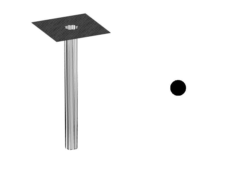
理想低通滤波器

在以原点为圆心，以$D_0$为半径的圆内无衰减通过所有频率，而在圆外切断所有频率的二维低通滤波器，称为理想低通滤波器(ILPF)，定义为
$$y=\begin{cases}
1,\quad D(x,y)\leq 0\
0, \quad D(x,y) > 0
\end{cases}$$
$D_0$是一个常数，D(u,v)是频率域中心点(u,v)与频率矩形中心的距离，即
$$ D(u,v)=\lbrack{(u-\frac{P}{2})^2+(v-\frac{Q}{2})^2}\rbrack^\frac{1}{2} $$
过渡点称为截止频率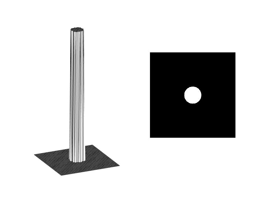

布特沃斯低通滤波器

截止频率位于距原点$D_0$处的n阶布特沃斯低通滤波器(BLPF)的传递函数的定义为:
$$H(u,v)=\frac{1}{1+{[D(u,v)/D_0]}^{2n}}$$
截止频率点是当D(u,v) = $D_0$时的点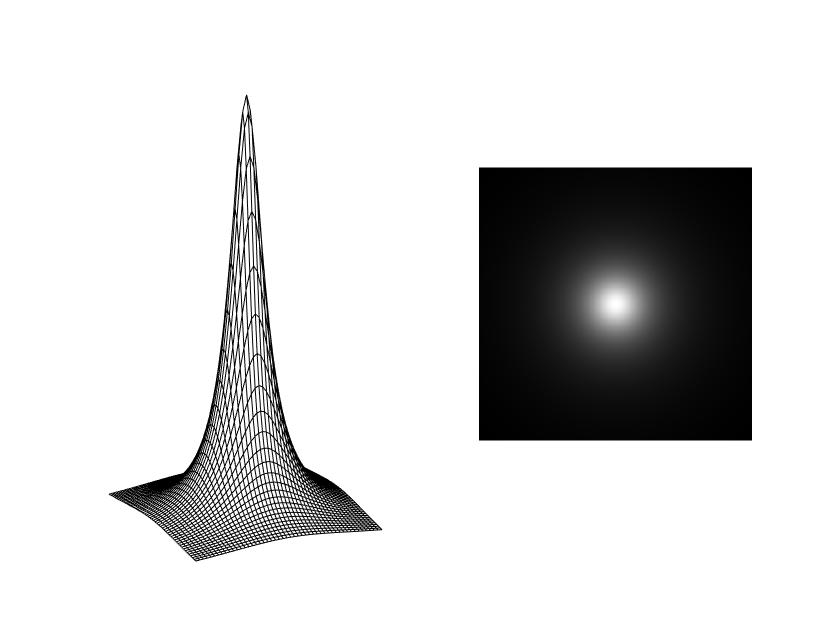

高斯低通滤波器

二维形式:
$$H(u,v) = e^{-D^2(u,v)/2{D_0}^2} $$
$D_0$ 是截止频率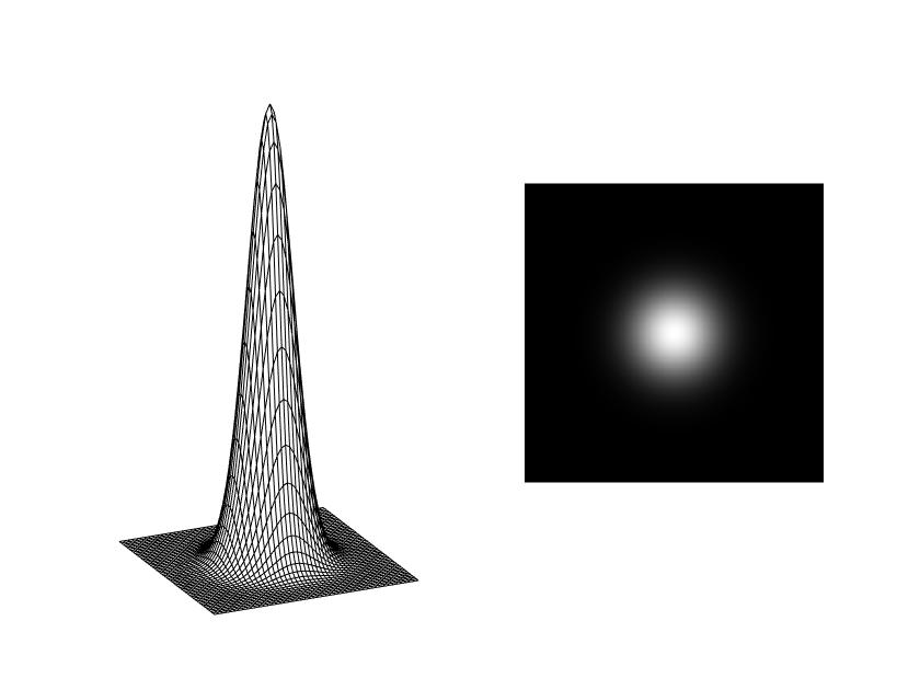

使用低通滤波器平滑图像

1. 高斯低通滤波器

f = imread('1.jpg');
f = rgb2gray(f);
[f, revertclass] = tofloat(f);
PQ = paddedsize(size(f));
[U, V] = dftuv(PQ(1), PQ(2));
D = hypot(U, V);
D0 = 0.05*PQ(2);
F = fft2(f, PQ(1), PQ(2));
H = exp(-(D .^ 2)/(2 * (D0^2))); %高斯低通滤波器
g = dftfilt(f, H);
g = revertclass(g);
figure, imshow(fftshift(H));
figure, imshow(log(1 + abs(fftshift(F))), [])
figure, imshow(g);

滤波结果：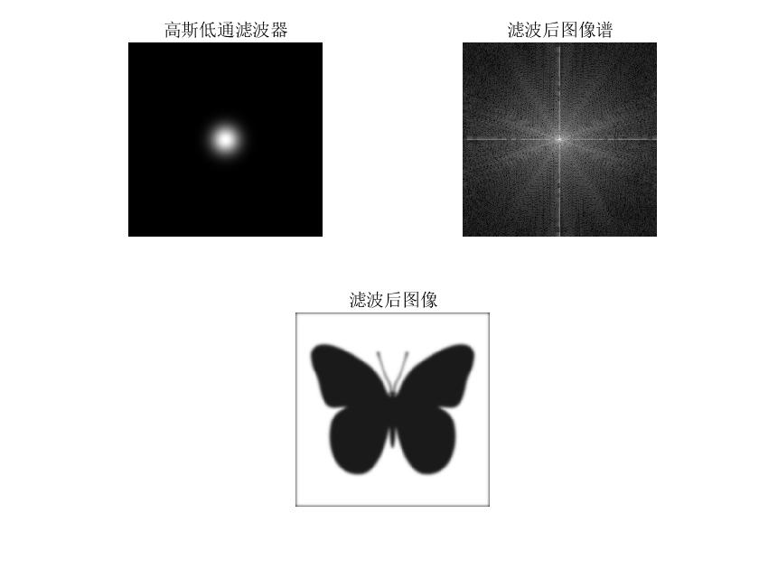

除了之前说的几个M函数外，还需要用到dftfilt()函数

function g=dftfilt(f,H)
%DFTFILT Performs frequency domain filtering.
%   G=DFTFILT(F,H) filters F in the frequency domain using the
%   filter transfer function H. The output, G, is the filtered
%   image, which has the same size as F. DFTFILT automatically pads
%   F to be the same size as H. Function PADDEDSIZE can be used
%   to determine an appropriate size for H.
%
%   DFTFILT assumes that F is real and that H is a real, uncentered,
%   circularly-symmetric filter function.

%Obtain the FFT of the padded input.
F=fft2(f,size(H,1),size(H,2));

%Perform filtering.
g=real(ifft2(H.*F));

%Crop to original size.
g=g(1:size(f,1),1:size(f,2));

2. Butterworth滤波

该函数输入为灰度图像，自由设置截止频率$D_0$和BLPF的阶数n，输出为滤波后的图像(已归一化到[0,255])

function [image_out] = Bfilter(image_in, D0, N)
% Butterworth滤波器，在频率域进行滤波
% 输入为需要进行滤波的灰度图像，Butterworth滤波器的截止频率D0，阶数N
% 输出为滤波之后的灰度图像

[m, n] = size(image_in);
P = 2 * m;
Q = 2 * n;

fp = zeros(P, Q);
%对图像填充0,并且乘以(-1)^(x+y) 以移到变换中心
for i = 1 : m
    for j = 1 : n
        fp(i, j) = double(image_in(i, j)) * (-1)^(i+j);
    end
end
% 对填充后的图像进行傅里叶变换
F1 = fft2(fp);

% 生成Butterworth滤波函数，中心在(m+1,n+1)
Bw = zeros(P, Q);
a = D0^(2 * N);
for u = 1 : P
    for v = 1 : Q
        temp = (u-(m+1.0))^2 + (v-(n+1.0))^2;
        Bw(u, v) = 1 / (1 + (temp^N) / a);
    end
end

%进行滤波
G = F1 .* Bw;

% 反傅里叶变换
gp = ifft2(G);

% 处理得到的图像
image_out = zeros(m, n, 'uint8');
gp = real(gp);
g = zeros(m, n);
for i = 1 : m
    for j = 1 : n
        g(i, j) = gp(i, j) * (-1)^(i+j);

    end
end
mmax = max(g(:));
mmin = min(g(:));
range = mmax-mmin;
for i = 1 : m
    for j = 1 : n
        image_out(i,j) = uint8(255 * (g(i, j)-mmin) / range);
    end
end
end

测试BLPF的阶数为2,截止频率分别为10,40,80,150,450

clear all;
close all;
clc;

image1 = imread('2.jpg');

image2 = Bfilter(image1, 10, 2);
image3 = Bfilter(image1, 40, 2);
image4 = Bfilter(image1, 80, 2);
image5 = Bfilter(image1, 150, 2);
image6 = Bfilter(image1, 450, 2);

% 显示图像
subplot(2,3,1), imshow(image1), title('原图像');
subplot(2,3,2), imshow(image2), title('D0 = 10, n = 2');
subplot(2,3,3), imshow(image3), title('D0 = 40, n = 2');
subplot(2,3,4), imshow(image4), title('D0 = 80, n = 2');
subplot(2,3,5), imshow(image5), title('D0 = 150, n = 2');
subplot(2,3,6), imshow(image6), title('D0 = 450, n = 2');

滤波结果如下: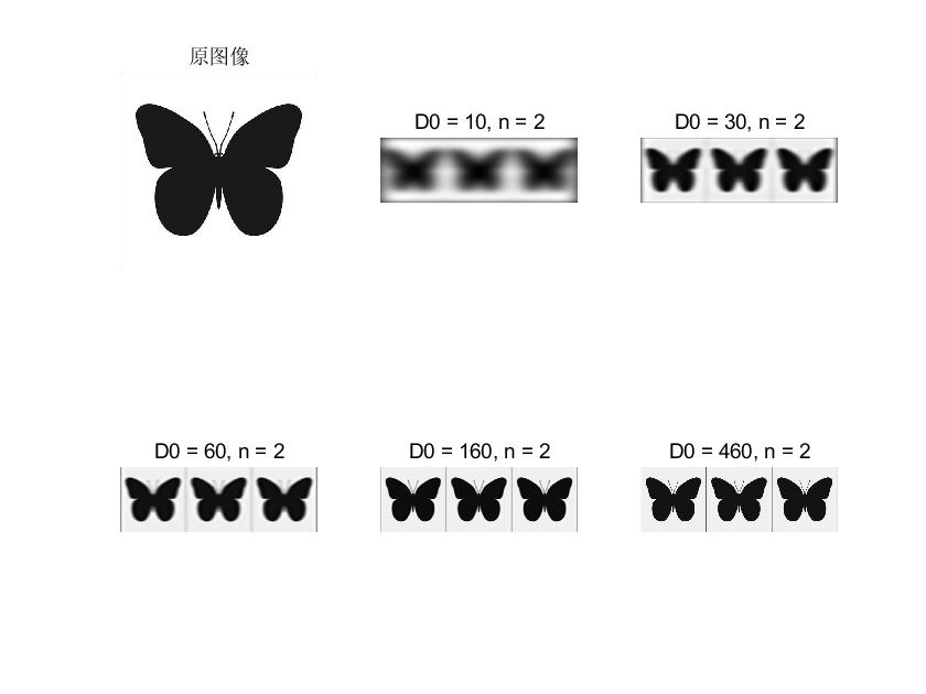

分析结果:

模糊的平滑过渡是截止频率增大的函数
滤波后输出三副连续的色图，原因是rgb图像的分三次呈现
一副彩图是由三色组成,红绿蓝三色，图像读取到matlab后，有三个参数m × n × 3, 代表的是三色叠加，处理之后的图将三色展开分别呈现了，所以才会出现三副连续的色图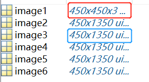

换成彩色图可以明显看到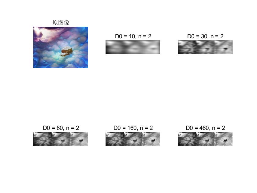

高通滤波器

图像的锐化可以在频率与通过高通滤波器来实现
一个高通滤波器可以由一个低通滤波器来实现:
$$H_{HP}(u,v)=1-H_{LP}(u,v)$$
被低通滤波器衰减的频率可以通过高通滤波器

理想高通滤波器

二维理想高通滤波器可以定义为
$$ H(u,v)=\begin{cases}
1,\quad D(u,v)\leq D_0\
0,\quad D(u,v)>D_0
\end{cases}
$$

布特沃斯高通滤波器

截止频率为$D_0$的n阶布特沃斯高通滤波器(BHPF)的定义为:
$$ H(u,v)=\frac{1}{1+[D_0/D(u,v)]^{2n}}$$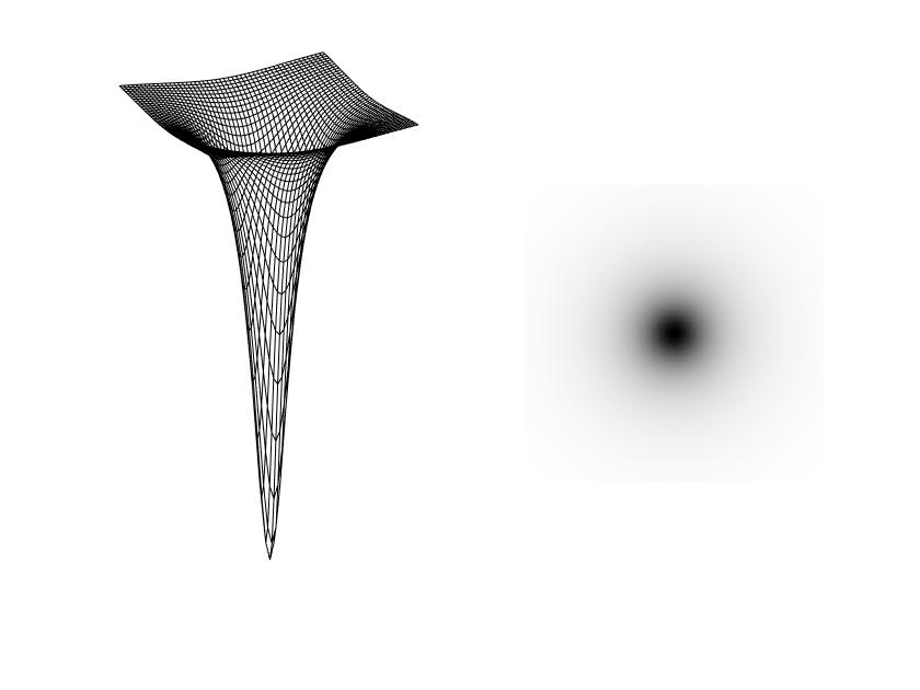

高斯高通滤波器

截止频率处在距频率矩形中心距离为$D_0$的高斯高通滤波器(GHPF)的传递函数如下:
$$H(u,v)=1-e^{-D^2(u,v)/2D_0^2}$$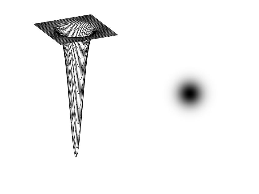

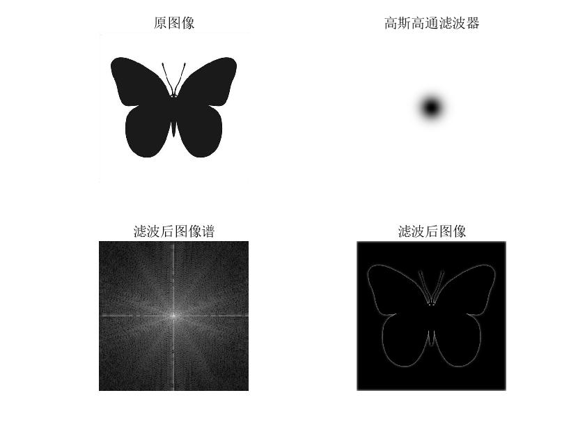
使用高通滤波器锐化图像

使用高通滤波器来锐化图像，与平滑图像类似，只是将低通滤波器换成了高通滤波器，具体步骤不再赘述

f = imread('1.jpg');
f = rgb2gray(f);
[f, revertclass] = tofloat(f);
PQ = paddedsize(size(f));
[U, V] = dftuv(PQ(1), PQ(2));
D = hypot(U, V);
D0 = 0.05*PQ(1);
F = fft2(f, PQ(1), PQ(2));
H = hpfilter('gaussian',PQ(1), PQ(2), D0);
g = dftfilt(f, H);
g = revertclass(g);
figure(1)
subplot(2,2,1);
imshow(f,[]);
title('原图像')
subplot(2,2,2);
imshow(fftshift(H));
title('高斯高通滤波器');
subplot(2,2,3);
imshow(log(1 + abs(fftshift(F))), [])
title('滤波后图像谱');
subplot(2,2,4);
imshow(g);
title('滤波后图像');

同样这里需要的是高通滤波函数hpfilter()

function [H] = hpfilter(type,M,N,D0,n)
%HPFILTER Computes freq. domain highpass filters
%        THIS IS NOT A STANDARD MATLAB FUNCTION
%        H = hpfilter (type,M,N,D0,n) creates the
%        transfer function of a highpass filter, H, of
%        the specified type and size MxN. Possible
%        values for type, D0, and n are:
%
%        'ideal'                Ideal highpass filter with
%                        cutoff frequency D0. If
%                        supplied, n is ignored.
%        'btw'                Butterworth highpass filter
%                        of order n, and cutoff D0.
%        'gaussn'            Gaussian highpass filter with
%                        cutoff (standard deviation)D0.
%                        If supplied, n is ignored.
%        M and N should be even numbers for DFT
%        filtering.
%
%        Class support: double, uint8, uint16
%        The output is of class double

%       The transfer function Hhp of a highpass filter
%       is 1 - Hlp, where Hlp is the transfer function of
%       the corresponding lowpass filter.  Thus, we can
%       use function lpfilter to generate highpass filters

%       If filter is btw, make sure that n is provided
%       Otherwise, pass n=1 as an arbitrary value to
%       prevent error message

if nargin == 4
    n = 1; %default value of n
end

Hlp = lpfilter(type,M,N,D0,n);
H = 1 - Hlp;

%       End of function

锐化结果: